


“How does product design work in an exchange?”
Having worked with exchange-traded derivatives throughout my career, this is a question I occasionally struggle to explain to others.
And perhaps that is not surprising.
In a typical Derivatives 101 class, we begin with forwards, futures, options and swaps. Much of the discussion then focuses on pricing: given an underlying asset, a payoff and a set of assumptions, what should the derivative be worth?
Many classical examples are also framed from the perspective of an over-the-counter (“OTC”) transaction between an investor and a bank.
The exchange itself rarely comes into the picture.
But before a derivative can be priced, someone first has to design it.
What exactly is the underlying? What currency should the contract be denominated in? How should it settle? When can the option be exercised? How should the payoff work? And how should gains and losses be margined?
These decisions eventually become something that may look deceptively mundane: the contract specifications.
Yet those specifications determine the risks embedded within a derivative and, in turn, how that derivative should be modelled and priced.
Exchange Traded Derivatives product design in itself is a form of financial engineering.
In this two-part article, I will introduce a stylized but practical framework for thinking about exchange-traded option design, and explore how each design choice eventually finds its way into quantitative modelling.
The 6 layers of Option Design
At its core, option valuation asks a relatively simple question: What is the discounted, risk-neutral expected value of the future payoff?
To answer that, we broadly need two things:
The dynamics of the underlying
The structure of the option payoff
The first tells us how the underlying asset may evolve through time.
A generic stochastic differential equation (“SDE”) can be written as
Once the possible future states of the underlying have been defined, the payoff structure tells us what the option is worth in each of those states.
(For more contextual knowledge, please refer to the previous article “Stochastic” is a difficult word.)
In practice, however, the contract specification contains several separate design decisions that determine both of these components.
I find it useful to break option design into six layers:
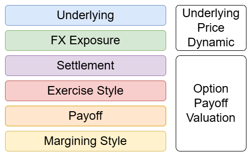
The first two primarily affect the dynamics of the underlying being priced, while the remaining layers primarily affect the valuation of the payoff.
This Part 1 focuses on the first three layers.
The framework is equally relevant to futures design, which is also why I begin directly with options: many of the underlying design considerations overlap.
Layer 1 - Underlying
The first question sounds obvious: What exactly is the option written on?
There are two dimensions to this question.
The first is the underlying asset itself.
Under the standard Black-Scholes framework, for example, the underlying follows a geometric Brownian motion. This implies that its log returns are normally distributed, while the asset price itself follows a lognormal distribution and remains strictly positive.
For many financial assets, this can be a useful approximation. But other markets exhibit characteristics that cannot always be represented adequately by a simple lognormal process.
Commodity markets are a good example.
Depending on the commodity, prices and forward curves may display characteristics such as:
mean reversion;
seasonality;
and, in some markets (e.g. electricity), the possibility of negative prices.
Even within financial markets, some assets may exhibit jumps that require richer price processes than simple diffusion models.
The point is not that one particular model is “correct”. Rather, the asset being chosen determines which behaviours the pricing model needs to accommodate.
Even the definition of the asset matters! In the case of an equity index, consideration of dividend reinvestment can impact pricing.
A price return index does not reinvest dividends paid by its constituents. Expected distributions therefore affect the economics of derivatives written on that index.
A total return index, on the other hand, reinvests those distributions into the index itself.
The two indices may contain exactly the same stocks, yet the treatment of dividends changes their level and return dynamics. The contract designer therefore needs to know precisely what exposure the derivative is intended to represent.
The second dimension is on the underlying instrument.
An option can be written on the actual underlying asset (“spot”/ “cash”), or on the futures on the underlying asset.
This distinction matters because the object being modelled has changed.
For a dividend-paying equity under the standard Black-Scholes assumptions, the risk-neutral spot dynamic can be written as
For an option on futures, the underlying is instead the futures price. Under the usual Black76 assumptions, the futures price is a martingale under the pricing measure:
The same economic exposure can therefore require a different pricing framework depending on what the option is legally written on.
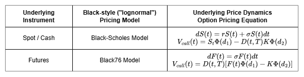
This distinction also has implications beyond valuation.
Where the exchange lists both the futures and its options, positions may form part of the same portfolio or trading strategy, potentially allowing risk offsets to be recognized within the margining framework.
I will return to margining in Part 2.
For now, the important point is:
Choosing the underlying does not merely determine what traders gain exposure to. It determines what price process needs to be modelled.
Layer 2 - FX Exposure
In many derivatives, we implicitly assume that the currency of the contract follows the currency of the underlying asset. But this does not always have to be the case.
Suppose an investor wants exposure to an asset denominated in a foreign currency. There are potentially two sources of risk:
Did the underlying asset rise or fall?
Did the foreign currency strengthen or weaken?
Product design determines whether the investor receives both risks or only the first.
There are several reasons why an exchange may want to separate the currency of the derivative from the currency of its underlying.
the product may cater to offshore investors whose portfolios are mainly accounted in USD instead of the local currency;
the local currency of the underlying asset is a restricted currency (e.g. Indian Rupee, Korean Won, Vietnamese Dong etc)
or the derivative may be intended to hedge a physical transaction denominated in one currency but benchmarked against an asset priced in another. (e.g. the ICE TTF 1st Line Futures, used for LNG trades in USD but benchmarked to the EUR-denominated Dutch TTF prices)
Two structures commonly used to deal with this are the compo and the quanto.
Compo (“Composite”)
A compo, or composite, derivative allows an investor to trade an asset denominated in a foreign currency while converting its value into another currency using the prevailing FX rate.
Suppose
St represents the foreign asset price;
Xt represents the FX rate converting the asset currency into the desired domestic currency.
The investor’s domestic-currency exposure then depends on XtSt . This means that both stochastic variables matter simultaneously:
where “f” in the subscript denotes foreign currency (the asset currency), and “d” in the subscript denotes the desired domestic currency.
There is one subtlety here: because the option is ultimately valued in the domestic currency, we need to express the foreign asset dynamics under the domestic pricing measure.
When the foreign asset dynamic is expressed under the domestic pricing measure, it acquires an FX correlation adjustment:
Combining this with the FX dynamics gives (Chin et al., 2017)
where
The compo adjustment creates the following impacts:
Once the asset is expressed in the desired domestic currency, the drift of the combined asset-and-FX exposure is governed by the domestic risk-free rate rather than the foreign risk-free rate.
the resulting volatility of the combined asset-and-FX exposure is a function of the asset volatility, FX volatility, and the correlation of the asset return and the FX
Because both the FX dynamics and the asset dynamics are being priced in, the holder of a compo derivative will need to actively hedge the FX exposure.
Quanto
A quanto takes a different approach. It gives investors exposure to the return of an asset denominated in a foreign currency without directly exposing them to movements in the FX rate.
Instead of allowing the exchange rate itself to determine the payoff, the product effectively fixes the currency conversion convention.
Under a common convention, the risk-neutral asset dynamic contains the quanto adjustment:
There are three things are worth noticing.
FX volatility no longer enters the diffusion term of the investor’s asset exposure directly.
FX still matters through the drift adjustment.
the absolute level of the spot FX rate is not what drives this adjustment. What matters is the volatility of FX and its correlation with the underlying asset.
The FX risk has not disappeared from the system. It has simply been transferred from the holder to the market maker. The market maker providing the fixed conversion must instead manage the interaction between the underlying asset and FX.
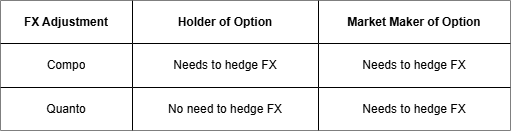
This is an important example of what derivatives design really means.
A compo and a quanto can reference exactly the same foreign asset. The difference lies in who bears the FX risk.
In the compo, the investor retains it.
In the quanto, that risk is transferred away from the investor and must instead be managed by the party providing the structure.
Neither structure is inherently superior. The right design depends on the intended users of the contract, the available hedging instruments and which risks those users are best equipped to manage.
From an exchange perspective, that matters greatly. The easier those risks are to understand, hedge and warehouse, the better the conditions for liquidity to develop.
Layer 3 - Settlement
The third layer asks a very practical question: What actually happens when the contract expires?
Broadly, derivatives can settle in two ways.
Physical settlement: The holder receives or delivers the underlying asset according to the contract specifications.
Cash settlement: Instead of exchanging the underlying, the economic gain or loss is converted into a cash payment between the counterparties
Physical settlement requires an ecosystem capable of supporting delivery, such as approved delivery locations, storage or warehouse arrangements, quality specifications, logistics, documentation and clearing procedures.
Cash settlement avoids much of that infrastructure by replacing delivery of the underlying with a monetary payment.
Under normal circumstances, the distinction may appear unimportant to the pricing of a derivative. However, in extreme circumstances, as seen in April 2020, the mechanics of settlement can become part of the price itself.
When a contract becomes very physical
On 20 April 2020, the May WTI crude oil futures contract settled at -$37.63/bbl. For the first time in history, the front-month WTI futures price had fallen deeply below zero!
Back then, COVID-19 had caused global oil demand to collapse while inventories continued accumulating. As the May WTI futures contract approached expiry, available storage capacity around its Cushing, Oklahoma delivery hub became increasingly scarce.
The long holders of the WTI futures are obliged to receive physical barrels if held to expiry. A long futures position was no longer simply just a financial exposure to the price of crude oil.
Traders with neither the infrastructure nor the intention to take delivery therefore needed to exit their positions. As available storage became increasingly scarce, the price required to convince someone else to assume that delivery obligation eventually fell below zero. In other words, holders were effectively willing to pay counterparties to take the long position from them.
And once futures prices became negative, another assumption broke. A lognormal model such as Black-76 cannot accommodate negative underlying prices.
Once the market demonstrated that crude oil futures could trade below zero, pricing and risk systems also needed to accommodate that possibility. CME Clearing sub-sequently switched specified option products to the Bachelier model to accommodate negative underlying futures prices (CME Clearing, 2020). ICE Futures Europe similar-ly announced that specified WTI options would use the Bachelier model for daily settlement (ICE Futures Europe, 2020).
The contract had not changed, but the observed domain of its price had, and the model had to change with it
This is perhaps the clearest example of the connection I wanted to illustrate through-out this article, that contract design can shape economic behaviour, and influence the quantitative models used in its pricing.
A decision about physical settlement ultimately affected not only delivery logistics, but the possible domain of the futures price, and therefore the option-pricing framework used around it.
Designing the contract before pricing it
What these three layers illustrate is that derivatives pricing does not begin with an equation. It begins with a set of design decisions.
What exactly is the underlying? That determines the price dynamics we need to model.
Who bears the currency risk? That determines whether FX volatility and asset-FX correlation enter the investor’s exposure, or are transferred elsewhere through a structure such as a quanto.
What happens when the contract expires? That determines whether physical constraints can become economically relevant to the pricing of the instrument itself.
This is why I think of derivatives product design as a form of financial engineering in the literal sense of the word. The contract specification is not merely documentation written after the product has been designed.
The specification is the design.
In Part 2, I will move from the underlying to the payoff itself: exercise style, payoff structure and margining. These layers determine how and when the option pays and how it should be valued.
References
Books
Chin, E., Nel, D. & Ólafsson, S. (2017). Problems and Solutions in Mathematical Finance, Volume 2: Equity Derivatives. Wiley.
de Weert, F. (2008). Exotic Options Trading. John Wiley & Sons.
Exchange Notices and Circulars
CME Clearing (2020). Switch to Bachelier Options Pricing Model – Effective April 22, 2020. Clearing Advisory No. 20-171, 21 April 2020. CME Group advisory
ICE Futures Europe (2020). Negative Pricing and Option Model Transition. Circular 20/057, 23 April 2020. ICE Futures Europe circular