


“What options would making this decision open up for you?”
It was during a breakfast that I was asked this question. It was from a mentor, someone in a senior position, while we were discussing an important decision to be made.
This question stayed with me.
We are constantly surrounded by options: what to have for lunch or which film to watch. Most of these choices are inexpensive and easily reversible. Sometimes, we have so many alternatives that the abundance itself becomes a problem that we complain about decision paralysis.
But as decisions become more consequential, the meaning of optionality changes.
Optionality is valuable because it preserves flexibility for tomorrow; It lets us act when circumstances are favorable without forcing us to act when they are not.
But it rarely comes for free. Preserving flexibility may require us to forgo immediate benefits, maintain excess capacity or pay for rights that we may never exercise. Recognizing valuable optionality therefore requires foresight and judgement.
It also raises a more difficult question:
How much should we be willing to pay to keep an option open?
That question was one of the central problems behind the development of modern quantitative finance.
How finance learned to price flexibility
One of the earliest rigorous mathematical theories of option valuation can be traced back to 1900, when Louis Bachelier published his thesis, “Théorie de la spéculation” (Bachelier, 1900).
Under Bachelier model, asset prices are modelled using arithmetic Brownian motion, where price changes over non-overlapping periods are independent and normally distributed. This mathematical model was elegant, ahead of its time, but remained largely overlooked for several decades.
In fact, Bachelier applied what we now recognize as Brownian motion to financial prices—five years before Einstein developed his physical theory of Brownian motion.
Over 70 years later, the Black-Scholes-Merton model was developed. The model assumed that the underlying asset followed geometric Brownian motion, producing a lognormal distribution of future prices. More importantly, it introduced a new way of thinking about valuation.
Rather than determining an option’s value by estimating how much return an investor would demand for bearing its risk, the model showed that an option could be replicated using a dynamically adjusted portfolio of the underlying asset and a risk-free money-market account.
If two positions produce the same future payoff, no-arbitrage implies that they must have the same value today. This replication argument also gives rise to risk-neutral valuation.
Under a risk-neutral framework, we do not attempt to estimate the real-world probability of every market outcome or the return demanded by every investor. Instead, we use market-consistent probabilities that allow the prices of tradable assets to be represented as discounted expected payoffs.
For a European call with a strike price of K, the value of the option can be expressed as the present value of its probability-weighted payoff at expiry:
The option’s value is the discounted risk-neutral expected value of its payoff at expiry
Subsequent models introduced more realistic assumptions, including stochastic volatility, jumps and more complex price dynamics. But the fundamental objective remained similar: to construct an internally consistent framework through which an uncertain, nonlinear future payoff could be valued today.
In other words, quantitative finance gave us a mathematical language for valuing flexibility.
But that flexibility does not always come in the form of a financial contract.
When the option is physical
“Suppose you have a cargo of liquefied natural gas. You can ship it to Europe or deliver it to Asia. How much is that flexibility worth?”
I was once asked this question during an interview for a commodity-quant role. I understood that the problem involved an option. But I had no idea how to structure it.
I didn’t manage to answer this question correctly. Fortunately, I still managed to secure the placement. And this became an essential part of my work as a physical commodity quant - the ability to identify, structure and value physical optionality.
Unlike financial options, physical optionalities are not traded instruments. These are operational flexibilities that are embedded in physical assets and commercial agreements: the ability to store, transport, transform or vary the quantity of a physical commodity depending on how market conditions evolve.
These flexibilities commonly appear across four dimensions: time, space, quantity and form (Trafigura, 2018).
Time
An owner of natural-gas storage has timing flexibility.
When gas prices are low, the owner may purchase gas and inject it into storage. The gas can then be withdrawn and sold during a later period when prices are higher.
The economic value of the storage asset is therefore not determined only by the absolute price of gas. It also depends on the relationship between prices across time.
Storage provides the ability to capture calendar spreads—but not the obligation to do so when the spread is insufficient to cover operating costs.
Space
Consider a cargo carrying one million barrels of oil that has loaded in Oman and is initially expected to sail towards Singapore.
While the vessel is in transit, demand in Europe increases and European prices rise relative to Asian prices. The trader may redirect the cargo towards Europe and replace the original Singapore delivery with another cargo sourced within Asia.
The ability to redirect the cargo creates a locational option. Its value depends on the spread between the two destination markets, adjusted for freight, timing, product specifications and other operating costs.
Quantity
Physical contracts frequently allow the quantity delivered to vary within a predefined range.
In LNG trading, for example, a contract may permit the delivered energy content to deviate by a specified percentage from the nominal amount. This is sometimes described as operational tolerance, or “optol.”
Suppose a trader has agreed to deliver 3.6 TBtu of LNG at a fixed price, with a quantity tolerance of plus or minus 10%.
When the contractual price is attractive relative to the spot market, the holder of the quantity flexibility may prefer to deliver more. When the contractual price is unattractive, the holder may prefer to deliver less and redirect the remaining volume elsewhere.
From the perspective of the party controlling the tolerance, the upward and downward flexibility may create call-like and put-like exposures. The precise payoff, however, depends on the contract, nomination rights and physical constraints.
Form
A gas-fired power plant converts natural gas into electricity.
The plant operator can choose to generate electricity when the power price exceeds the cost of the gas, emissions and other variable operating expenses. When the economics are unfavorable, the operator may reduce production or shut down the plant.
This conversion flexibility creates an option on the spark spread: the margin between the value of electricity produced and the cost of the inputs required to produce it.
Across all four dimensions, control of a physical asset can provide more than ownership of the commodity itself. It can provide the right to respond as market conditions change.
That right has economic value.
Optionality as a commercial currency
In commodity trading, physical optionalities often function as bargaining chips in negotiations (“commercial currencies”).
A buyer may surrender some contractual flexibility in exchange for a better flat price. A seller may offer a discount to gain destination rights, quantity flexibility or timing discretion that complements the rest of its portfolio.
These concessions are not merely legal details.
A destination clause, loading window or quantity tolerance may appear minor when a contract is signed. But under the right market conditions, it can become highly valuable.
The challenge is that not all physical flexibilities are equally easy to recognize or value.
Some are closely linked to observable market prices and can be approximated using existing financial instruments. Others depend on operational conditions, private information or non-traded risks for which no unique market value exists.
During my time as a commodity quant, I came to think about physical optionality across three practical dimensions.
Observability: Are the relevant market prices and costs observable?
Modelability: Can the payoff and its principal risk drivers be represented credibly?
Hedgeability: Can a substantial portion of the exposure be offset using sufficiently liquid financial instruments?
Above all, physical optionality must be exercisable whenever the opportunity arises. If one does not own full exercise rights, then the flexibility is not real.
A physical flexibility becomes especially useful as a commercial currency when it performs well across all these dimensions.
I think of this subset as tradable physical optionality.
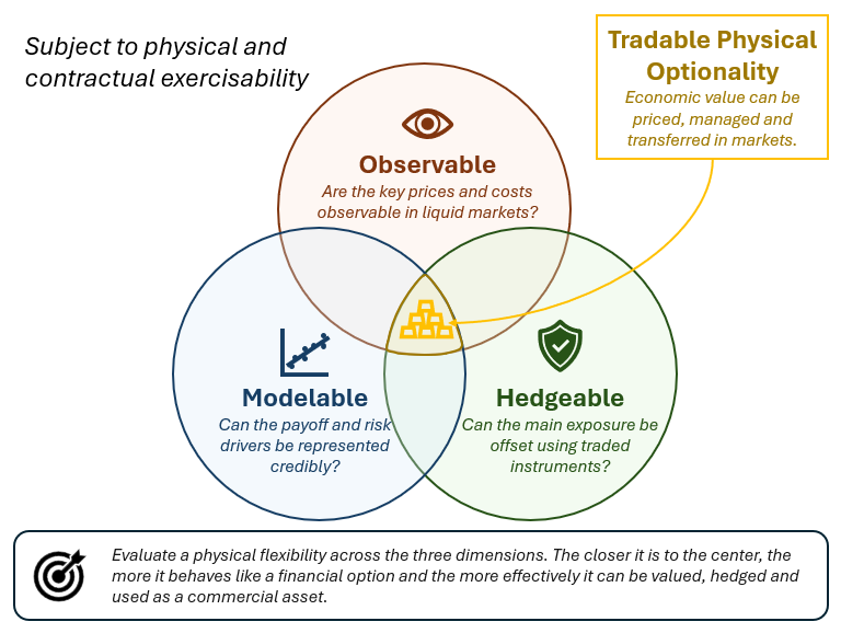
Framework for identifying tradable physical optionality.
A tradable physical optionality is an operational flexibility whose principal economic exposures can be approximated, valued and substantially hedged using sufficiently liquid instruments in the market.
Replication will rarely be perfect due to basis risk, liquidity constraints, logistical uncertainty and contractual complexity. However, an optionality that is close to a tradable physical optionality is highly valuable because:
It makes the optionality easier to value.
It allows the holder to manage or transfer part of the exposure.
It allows the optionality to be used more deliberately in commercial negotiations.
Flexibilities that do not meet these conditions are not necessarily less valuable, but their value may be harder to measure, hedge and monetize, thus less effective as bargaining chips.
Revisiting the interview
Going back to the interview question, how do we value such optionality?
By now, we should have identified this to be an optionality on “space”. More specifically, this is destination flexibility: a locational option on the relative netback between Europe and Asia.
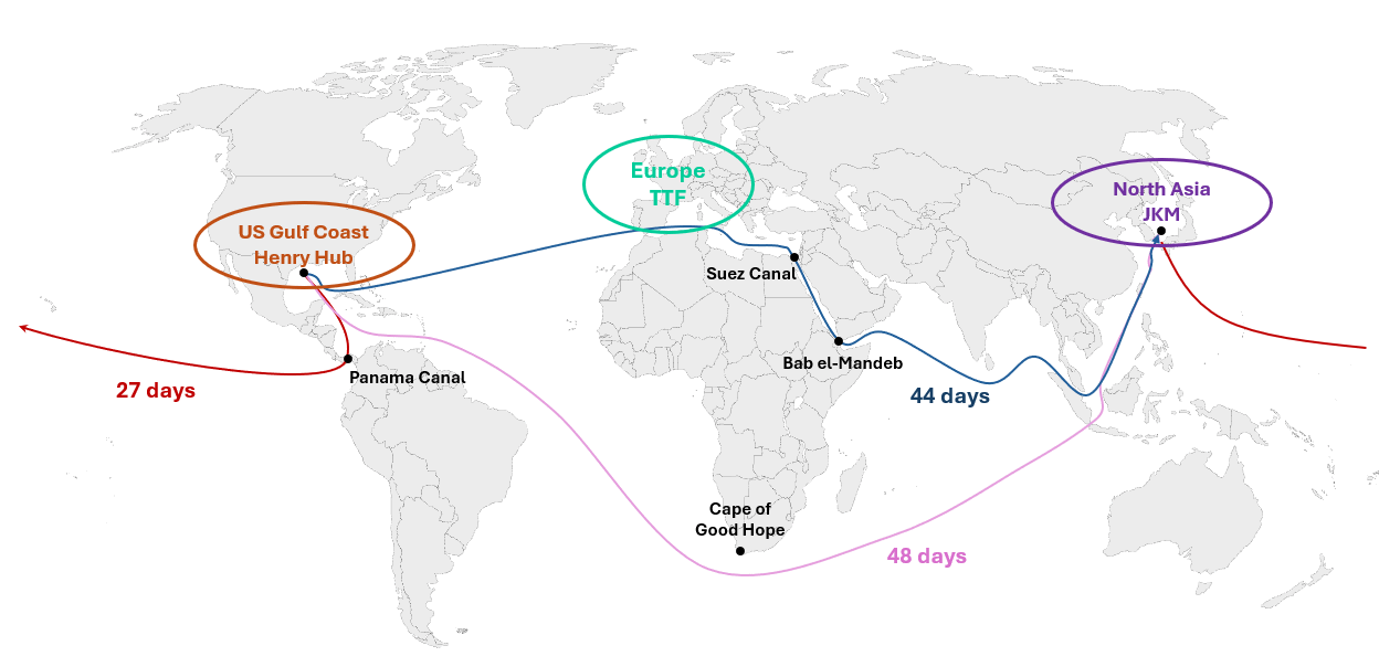
Illustrative LNG routes and regional pricing references. Schematic by the author; routes and transit times are approximate.
Suppose an LNG cargo originates from the United States Gulf Coast and can be delivered either to Europe or Northeast Asia. For a simplified illustration, we can use
TTF as the liquid reference for European gas value;
JKM as the delivered LNG benchmark for Northeast Asia; and
Henry Hub as a reference for US feed-gas cost.
For simplicity, assume that all benchmark prices and operating costs have been converted into a common currency and energy unit.
The payoff of delivering the cargo to Europe can be represented as a simplified netback:
where KUS→EU represents the operating costs of delivering the cargo from the US Gulf Coast to Europe.
Similarly, the payoff of delivering the cargo to Asia can be written as
If Europe is the default destination, the incremental payoff of having the right to divert the cargo to Asia is
This payoff represents the value of the cargo’s destination flexibility.
Therefore, the value of the cargo Vc is:
At first glance, this resembles an option on the spread between JKM and TTF, with the difference in operating costs acting like a strike.
But identifying the payoff is only the beginning.
The art of valuing physical optionality is in how one models the price dynamics of the commodity. One approach is to model each leg by itself and establishing a joint distribution to preserve the statistical relationship between the two moving parts. Another is to model the spread directly using the Bachelier model (Carmona & Durrleman, 2003).
The correlation between the two markets is particularly important. If European and Asian prices move almost perfectly together, the value of switching between the destinations may be limited. If the relative spread is volatile, destination flexibility becomes more valuable.
Since there are futures on Dutch TTF Natural Gas and on LNG JKM, both listed on the Intercontinental Exchange, this optionality can be partially replicated and hedged with the listed futures, allowing traders to trade around the optionality.
Where the financial model ends
The economic exposures associated with physical optionalities can resemble traded instruments such as calendar spread option (time), locational spread option (space), option straddle (quantity), or spark spread option (form).
It would be natural to think about having some of these spread options become listed financial options.
In fact, we do see some of these options being listed on exchanges. In 2023, ICE announced an expanded offering of TTF natural-gas calendar spread options (Intercontinental Exchange, Inc., 2023).
However, there are several practical issues with using listed spread options to replicate physical optionality:
Different traders face different operating costs and financing assumptions, which could lead to high customization and fragmenting liquidity.
The non-zero strike that encapsulates operating costs can be stochastic in nature - operating costs include freight, which has its own price dynamics with high volatility and jumps that cannot be ignored.
The exercisability of physical optionality goes beyond pure economics - optionality can be destroyed if it is no longer physically possible to capture.
The last point is extremely important. An attractive locational spread may remain economically in-the-money, yet become impossible to capture if the required route is unavailable. In that situation, the spread has not necessarily moved against the trader. Instead, the physical option has lost its exercisability. This is an event that is beyond simple price movement, a risk that may be difficult or impossible to hedge completely using conventional price-based derivatives.
This creates an important separation between economic moneyness and physical exercisability.
A model can tell us whether an action appears profitable. But it cannot guarantee that the action remains possible.
That is why valuing physical optionality often requires more than conventional option-pricing theory. Depending on the asset, the problem may require considerations on logistical constraints and repeated decisions across time. It may involve more advanced techniques, such as dynamic programming and stochastic optimal control.
For me, that is what made commodity quantitative work so compelling. The models were sophisticated, and the problems were grounded in the physical world and real commercial decisions.
Optionality as a life principle
I can’t remember my response to my mentor, or if the decision I made did provide me with more options in the end.
But his question changed how I evaluate decisions.
My understanding of optionality has gradually moved beyond the field of financial derivatives or commodity trading. It has become a broader way of thinking
Optionality asks us to consider not only what a decision gives us today, but also what it allows us to do tomorrow.
Sometimes, the right decision is to commit decisively. Keeping every option open can become expensive, distracting and ultimately paralyzing.
But at other times, flexibility is worth paying for—particularly when uncertainty is high, new information is likely to arrive and the future opportunities are asymmetric.
The central lesson is not that we should always maximize the number of choices available to us. It is that choices themselves have value, and giving them up has a cost.
Financial models help us make that intuition explicit. They show how uncertainty, time and asymmetric payoffs can turn flexibility into something economically valuable.
And in the physical world, some of the most important options may be hidden in places we do not immediately recognize: inside a storage facility, a cargo route, a power plant, a commercial contract—or an important decision made over breakfast.
References
Bachelier, L. (1900). Théorie de la spéculation. Annales scientifiques de l’École Normale Supérieure, 17, 21–86.
Carmona, R., & Durrleman, V. (2003). Pricing and hedging spread options. SIAM Review, 45(4), 627–685. https://doi.org/10.1137/S0036144503424798
Intercontinental Exchange, Inc. (2023, October 30). ICE expands global energy portfolio with the launch of TTF natural gas calendar spread options [Press release]. https://ir.theice.com/press/news-details/2023/ICE-Expands-Global-Energy-Portfolio-With-the-Launch-of-TTF-Natural-Gas-Calendar-Spread-Options/default.aspx
Trafigura. (2018). Commodities demystified: A guide to trading and the global supply chain (2nd ed.). https://www.commoditiesdemystified.info/pdf/CommoditiesDemystified-en.pdf