


I have always believed that one of the best tests of understanding is whether you can explain something simply. Teaching, to me, is one of the most effective ways to fully understand and master a subject matter.
Therefore, I make it challenge to start Quant Simplified. By curating content around the fundamentals of quantitative finance, it challenges me to gain deeper understanding of essential concepts in the field. It is also way to help aspiring quants develop an intuition for concepts that can otherwise seem unnecessarily intimidating.
And few words in quantitative finance sound quite as intimidating as stochastic.
The inspiration for this article came from a conversation about what quants actually do, and how we explain complicated ideas to people without a quantitative background.
In that conversation, I was asked:
What is Itô’s Lemma, and why does anyone in trading or option pricing care about it?
There is, of course, a mathematical answer to that question.
But before getting there, there is a much simpler story. It begins with tossing a coin.
“Stochastic” is a difficult word
When I first started studying quantitative finance, stochastic calculus was one of the topics I found most intimidating. Even the word sounds complicated and hard to pronounce!
Its underlying idea, however, is much simpler: stochastic means that randomness is involved. And once randomness enters the picture, probability follows naturally.
Consider a simple game. You have a fair coin. Every time you toss it:
- Heads (‘H’) earns you +1
- Tails (‘T’) earns you −1
You are asked to play this for many rounds and you are to accumulate the points as you progress into the game.
A few useful concepts immediately appear.
Sample space: it is a set of possible outcomes of the random game. In our case, it’s ‘Head’ (‘H’) or ‘Tail’ (‘T’)
Random variable: it is a numerical value that is assigned to an outcome. Here, the random variable takes a discrete value of either -1 or 1. The score that we earn is our random variable
If we only played one turn, our sample space will be limited to 2 outcomes, and our random variable will be restricted to 2 possible values.
Now suppose we keep playing. After every toss, we record our cumulative score. The value of that score is uncertain before each toss, but it evolves through time according to the outcomes of the game.
That collection of random variables indexed by time is what we call a stochastic process.

Over ten tosses, the path might look rather uninteresting, or perhaps rather unlucky! But what if we repeat the game a thousand times?

That is better, I managed to get a positive score! But wait… Now something interesting starts to appear. Ignoring the terminal number for a moment, doesn’t this path look like how a stock price would move?
Asset price dynamics follow a stochastic process
Just like our cumulative score from the coin tosses, the price of an asset is a random variable, and its future price is uncertain.
We do not know today exactly where a stock, commodity or exchange rate will trade tomorrow, next month or next year. That uncertainty is one reason stochastic processes are so important in finance.
If we want to value derivatives whose future payouts depend on an asset price, we first need some description of how that asset price might evolve.
That immediately raises two questions:
What probability distribution should describe the possible outcomes?
What parameters should that distribution have?
The first question is arguably the harder one.
With our coin toss, we knew the probabilities beforehand: 50% heads and 50% tails. However, financial markets give us no such luxury. The true probability distribution of future returns is unknown. We therefore need to make assumptions and choose an appropriate model.
The most common starting point assumes that continuously compounded returns are normally distributed. If log returns are normally distributed, the corresponding asset price is lognormally distributed.
This gives us one of the most recognizable processes in quantitative finance: Geometric Brownian Motion.
Its stochastic differential equation is
where:
St is the asset price,
μ is its drift,
σ is its volatility,
Wt is a Wiener process.
This equation contains two very different components - the drift and the diffusion.
The drift describes the systematic direction of the process, while the diffusion introduces randomness.
The Wiener process itself has normally distributed increments. Over a small interval of time dt, that random shock scales approximately with dt.
And this deceptively simple equation becomes the starting point for a large part of classical derivatives pricing.
Now, we have decided what distribution to describe the future outcome, we are now into the second problem - how do we define the parameters?
Which drift should we use?
There is an immediate problem. What should μ actually be?
Suppose Investor A expects an asset to appreciate at 5% per year. Investor B believes the same asset will fall by 2%.
Both might have sophisticated models supporting their views. But before the future unfolds, we cannot know which forecast is correct.
These forecasts belong to what quants generally call the ‘real world’ measure, or the P-measure: a description of probabilities as they are believed to operate in the real world.
This creates an obvious difficulty for derivatives pricing. If every investor has a different forecast for the asset’s expected return, must every investor therefore have a completely different option price?
Fortunately, under certain conditions, no. And this is where risk-neutral pricing enters the picture.
Risk-neutrality
One of the most powerful ideas in derivatives pricing is that, when risks can be replicated or hedged using traded assets and the market is free of arbitrage, we can value derivatives under a different probability measure.
This is what we commonly refer to as the risk-neutral measure, or the Q-measure. Under the risk-neutral measure, the expected return of a tradable asset is no longer determined by an investor’s personal forecast of its future performance.
For many assets, one can rely on risk-neutral pricing to determine the drift. Without going too much into the details, the key idea is that if we can hedge a portfolio perfectly, the expected value of the portfolio measured with respect to a reference asset would remain the same as the initial value of the portfolio w.r.t. that reference asset.
where t<T, Vt is the value of the portfolio, Nt is the value of the reference asset, and QN is the measure associated with reference asset N.
This reference asset has a unique name in quantitative finance, and it is known as the numeraire. The numeraire has to meet certain conditions; for one it must be a tradable asset, and it must be strictly positive.
As it turns out, to replicate and hedge a forward contract or an option contract, a common choice of numeraire is the money-market account. When the money-market account is used as the numeraire, appropriately discounted tradable asset prices behave as martingales under the associated risk-neutral measure.
For simplicity, assuming a non-dividend paying equity, the drift in the SDE under Q-measure becomes simply the risk free rate of interest in the currency of the underlying asset.
Therefore, derivatives pricing can often be separated from forecasting the underlying asset’s actual expected return.
Now we return to the original question: So where does Itô’s Lemma come in?
Ordinary calculus gives us rules for understanding how functions change. But stochastic processes behave differently.
A Wiener process is continuous but nowhere differentiable in the ordinary sense, so the usual rules of calculus cannot simply be applied unchanged.
Itô’s Lemma, which can be derived from a stochastic extension of Taylor expansion, allows us to transform stochastic processes and, in some cases, solve their SDEs. More importantly for option pricing, it tells us how a derivative value V(S,t) evolves when the underlying asset follows a stochastic process.
Option pricing = pricing a distribution of payoffs
The bulk of this article has been explaining what is a stochastic process and how we determine the parameters of the assumed distribution. We have not explained why we need to model the asset price as a stochastic process. The answer is rather simple — it is because of the non-linearity of the option contract payout.
Consider a forward contract.
Suppose an asset trades at S0 today. If we can buy the asset, finance that purchase and account for any income generated by holding it, we can construct the economics of a forward synthetically.
For an equity paying a continuous dividend yield q,
Notice what is missing. We did not need to know the stock’s volatility, nor do we need to predict whether it would rise or fall tomorrow. That is possible because the forward payoff is linear in the underlying price.
But an option is different. Option is non-linear.
Now consider a call option. At expiry, its payoff is
If the asset finishes above the strike K, the option has value. Otherwise, if the asset finishes below the strike, the holder can simply walk away and the payoff is zero.
That asymmetry is the defining feature of optionality. And knowing only the average future asset price is no longer enough.
That asymmetry gives the option positive value to the buyer. The seller therefore requires compensation — an option premium — for taking on the contingent payoff
To determine this premium amount, one needs to evaluate the probability of being exercised against — meaning the probability that the underlying price would exceed the strike price level— and the payoffs.
Option pricing is therefore not simply about estimating the probability of exercise. It is about evaluating an entire distribution of possible payoffs.
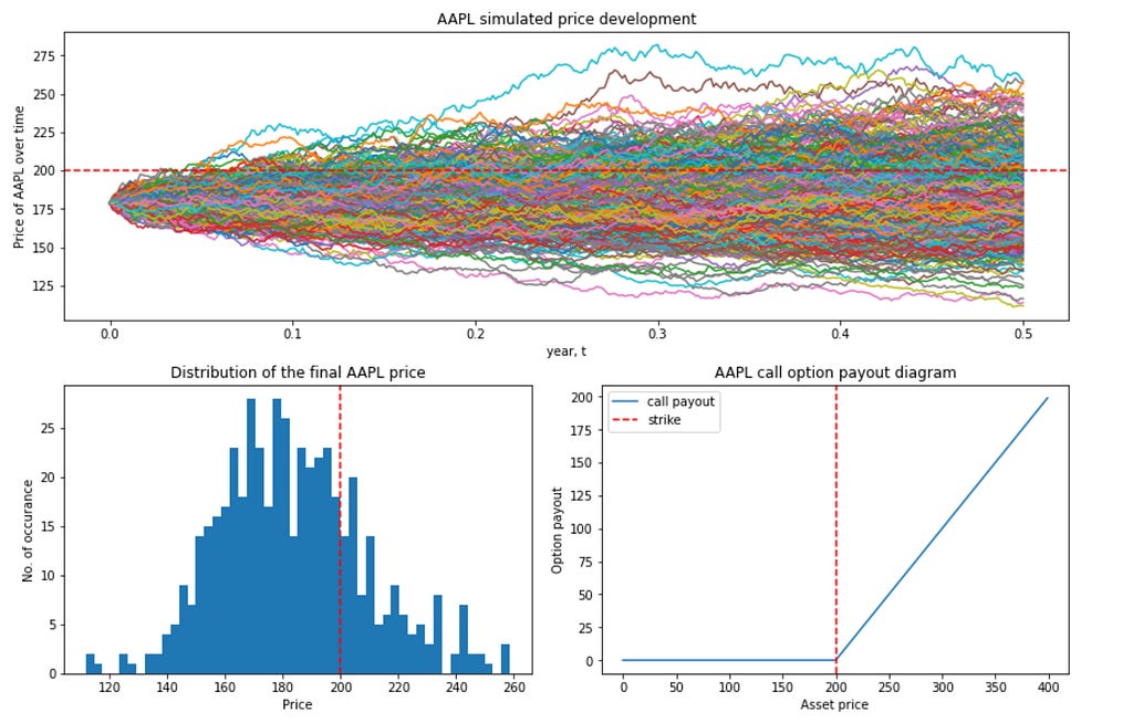
This is how stochastic process and calculus are relevant in quantitative finance — it allows us to price derivatives that are non-linear.
If one further expands on the equation below, one would arrive at the Black-Scholes option pricing equation. This also explains why there are cumulative distribution functions within the BS equation. It is about evaluating an entire distribution of possible payoffs.
Now imagine two possible worlds. In both worlds, the expected future stock price is exactly the same.
In one world, the stock barely moves. But in the other, its possible outcomes are spread over a much wider range. The call option will generally be worth more in the second world.
Why? Because the upside can keep growing while the downside payoff is floored at zero. That convexity is why volatility matters.
The key is volatility
We have dealt with the drift with risk-neutral measure. We are now left with the remaining important point — volatility.
Volatility determines how widely the possible future outcomes spread. All else equal, greater volatility generally increases the value of a vanilla option.
For a call option, a wider distribution creates more opportunities for large positive payoffs, while the downside payoff remains bounded at zero.
But there is one obvious problem: what volatility should we use?
Historical volatility is one possibility. Another possible candidate is implied volatility.
If there is a liquid options market, demand and supply would help determine a price level that reflects the market’s pricing of volatility, including expectations, supply and demand, and risk premia.
By using the market option prices, one could work in reverse with the BS equation to determine the volatility used — therefore this is called the “implied” volatility. This implied volatility could then be used, and one can adjust based on one’s own expectation of the volatility.
The real world is not that straightforward
Everything so far has deliberately simplified reality, which is useful for understanding the foundations. But it is equally important to understand where those foundations become insufficient.
First, asset returns do not behave exactly like the normal distribution assumed by the simplest Geometric Brownian Motion model.
Equity returns often exhibit skewness and fat tails, markets jump, and volatility changes through time. These features make Geometric Brownian Motion too simplistic for many real-world applications.
Second, implied volatility requires observable option prices. What happens when an options market is illiquid—or does not exist at all? Then volatility estimation becomes a considerably harder problem.
Finally, some risks cannot be perfectly replicated using traded instruments. Weather is an obvious example. Volatility itself also presents complications because it is not an ordinary cash asset that can simply be purchased and stored.
These complications are not failures of quantitative finance. They are the reason quantitative finance remains interesting.
Models simplify reality so that we can reason about it. The important thing is understanding what has been assumed, what the model gives us, and where those assumptions begin to break down.
So what does “stochastic” really mean?
We started by tossing a coin. That simple random walk gave us a way to think about uncertainty evolving through time.
From there, we moved to stochastic asset-price dynamics. Those dynamics led us to probability distributions.
Risk-neutral pricing allowed us to price derivatives without having to agree on the asset’s actual expected return.
Itô’s Lemma gave us a way to describe how derivatives of stochastic variables evolve, forming a bridge from asset-price dynamics to option pricing.
And the non-linear payoff of an option showed us why the entire distribution—not just the expected asset price—matters.
That is a lot of quantitative finance hiding behind one difficult word.
Stochastic — Still a difficult word to spell, but hopefully a little easier to understand.
This is the 2nd version of the article. Updated on 30th September 2026.